2. Photometric Data

In astronomy, there are two ways we can measure an object in the sky. One method that is expensive method is to construct a spectrum. A cheaper method is to take photometric measurements (i.e. putting the light into some number of bins).

2.1. Dust Extinction

As light travels through space to Earth, some of it get absorbed and scattered by the galatic dust. Light in the higher frequency is more affected, hence extinction causes an object to become redder. This gives the phonomena the name interstallar reddening.

The amount of extinction varies across the sky. For example, there is a lot of dust in the Milky Way band, as can be seen from the following reddening map, where red indicates a high level of extinction:

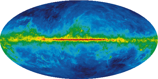
Figure 1: Galatic reddening map (Source: LAMBDA)

Thus we need to correct the photometric data for this bias.

2.1.1. SFD98 Correction Set

In the SDSS dataset (which will be used throughout the example notebooks), there are four columns labelled \(A_u\), \(A_g\), \(A_r\), \(A_i\), and \(A_z\). We will need to subtract these from the ugriz filter magnitudes. The corrected magnitudes will become smaller, corresponding a brighter flux (yes, the astronomical magnitude system is weird!). This set of correction is called SFD98, which has been the default choice in the astronomical community for a long time.

2.1.2. SF11 Correction Set

There is another variation called SF11, where there is one free paramter. In trying to refine the dust extinction estimates, we need to turn our attention to the \(E_{b1-b2}\) band instead of the A-band. Define the reference value

\[E_{B-V} = \dfrac{A_r}{2.751}\]

where \(A_r\) is from the SFD98 set. Then we can retrieve the SF11 estimates:

\[\begin{split}A'_u = E_{B-V} * 4.239 \\ A'_g = E_{B-V} * 3.303 \\ A'_r = E_{B-V} * 2.285 \\ A'_i = E_{B-V} * 1.698 \\ A'_z = E_{B-V} * 1.263\end{split}\]

As an aside, we can also recover the SFD98 estimates:

\[\begin{split}A_u = E_{B-V} * 5.155 \\ A_g = E_{B-V} * 3.793 \\ A_r = E_{B-V} * 2.751 \\ A_i = E_{B-V} * 2.086 \\ A_z = E_{B-V} * 1.479\end{split}\]

2.1.3. W14 Correction Set

In the most recent correction set from [W2014], we again start with

\[E_{B-V} = \dfrac{A_r}{2.751}\]

We now need to remap the \(E_{B-V}\) scale:

\[\begin{split}E_{B-V} \in [0,0.04] &\rightarrow E'_{B-V} = E_{B-V} \\ E_{B-V} \in [0.04,0.08] &\rightarrow E'_{B-V} = E_{B-V} + 0.5 * (E_{B-V} - 0.04) \\ E_{B-V} \in [0.08,+\infty] &\rightarrow E'_{B-V} = E_{B-V} + 0.02\end{split}\]

This allows us to calculate the W14 estimates:

\[\begin{split}A''_u = E'_{B-V} * 4.305 \\ A''_g = E'_{B-V} * 3.288 \\ A''_r = E'_{B-V} * 2.261 \\ A''_i = E'_{B-V} * 1.714 \\ A''_z = E'_{B-V} * 1.263\end{split}\]

References

[W2014]

Wolf, Christian. “Milky Way dust extinction measured with QSOs”. arXiv:1410.0109 [astro-ph.GA]